awips2/docs/python/map-resources-and-topography.md

The python-awips package provides access to the entire AWIPS Maps Database for use in Python GIS applications. Map objects are returned as Shapely geometries (Polygon, Point, MultiLineString, etc.) and can be easily plotted by Matplotlib, Cartopy, MetPy, and other packages.

Each map database table has a geometry field called the_geom, which can be used to spatially select map resources for any column of type geometry,

Notes

• This notebook requires: python-awips, numpy, matplotplib, cartopy, shapely

• Use datatype maps and addIdentifier('table', <postgres maps schema>) to define the map table: DataAccessLayer.changeEDEXHost("edex-cloud.unidata.ucar.edu") request = DataAccessLayer.newDataRequest('maps') request.addIdentifier('table', 'mapdata.county')

• Use request.setLocationNames() and request.addIdentifier() to spatially filter a map resource. In the example below, WFO ID BOU (Boulder, Colorado) is used to query counties within the BOU county watch area (CWA)

    request.addIdentifier('geomField', 'the_geom')
    request.addIdentifier('inLocation', 'true')
    request.addIdentifier('locationField', 'cwa')
    request.setLocationNames('BOU')
    request.addIdentifier('cwa', 'BOU')
  

See the Maps Database Reference Page for available database tables, column names, and types.

Note the geometry definition of the_geom for each data type, which can be Point, MultiPolygon, or MultiLineString.

Setup

from __future__ import print_function
from awips.dataaccess import DataAccessLayer
import matplotlib.pyplot as plt
import cartopy.crs as ccrs
import numpy as np
from cartopy.mpl.gridliner import LONGITUDE_FORMATTER, LATITUDE_FORMATTER
from cartopy.feature import ShapelyFeature,NaturalEarthFeature
from shapely.geometry import Polygon
from shapely.ops import cascaded_union

# Standard map plot
def make_map(bbox, projection=ccrs.PlateCarree()):
    fig, ax = plt.subplots(figsize=(12,12),
            subplot_kw=dict(projection=projection))
    ax.set_extent(bbox)
    ax.coastlines(resolution='50m')
    gl = ax.gridlines(draw_labels=True)
    gl.xlabels_top = gl.ylabels_right = False
    gl.xformatter = LONGITUDE_FORMATTER
    gl.yformatter = LATITUDE_FORMATTER
    return fig, ax

# Server, Data Request Type, and Database Table
DataAccessLayer.changeEDEXHost("edex-cloud.unidata.ucar.edu")
request = DataAccessLayer.newDataRequest('maps')
request.addIdentifier('table', 'mapdata.county')

Request County Boundaries for a WFO

• Use request.setParameters() to define fields to be returned by the request.

# Define a WFO ID for location
# tie this ID to the mapdata.county column "cwa" for filtering
request.setLocationNames('BOU')
request.addIdentifier('cwa', 'BOU')

# enable location filtering (inLocation)
# locationField is tied to the above cwa definition (BOU)
request.addIdentifier('geomField', 'the_geom')
request.addIdentifier('inLocation', 'true')
request.addIdentifier('locationField', 'cwa')

# This is essentially the same as "'"select count(*) from mapdata.cwa where cwa='BOU';" (=1)

# Get response and create dict of county geometries
response = DataAccessLayer.getGeometryData(request, [])
counties = np.array([])
for ob in response:
    counties = np.append(counties,ob.getGeometry())
print("Using " + str(len(counties)) + " county MultiPolygons")


%matplotlib inline
# All WFO counties merged to a single Polygon
merged_counties = cascaded_union(counties)
envelope = merged_counties.buffer(2)
boundaries=[merged_counties]

# Get bounds of this merged Polygon to use as buffered map extent
bounds = merged_counties.bounds
bbox=[bounds[0]-1,bounds[2]+1,bounds[1]-1.5,bounds[3]+1.5]


fig, ax = make_map(bbox=bbox)
# Plot political/state boundaries handled by Cartopy
political_boundaries = NaturalEarthFeature(category='cultural',
                               name='admin_0_boundary_lines_land',
                               scale='50m', facecolor='none')
states = NaturalEarthFeature(category='cultural',
                               name='admin_1_states_provinces_lines',
                               scale='50m', facecolor='none')
ax.add_feature(political_boundaries, linestyle='-', edgecolor='black')
ax.add_feature(states, linestyle='-', edgecolor='black',linewidth=2)

# Plot CWA counties
for i, geom in enumerate(counties):
    cbounds = Polygon(geom)
    intersection = cbounds.intersection
    geoms = (intersection(geom)
         for geom in counties
         if cbounds.intersects(geom))
    shape_feature = ShapelyFeature(geoms,ccrs.PlateCarree(), 
                        facecolor='none', linestyle="-",edgecolor='#86989B')
    ax.add_feature(shape_feature)

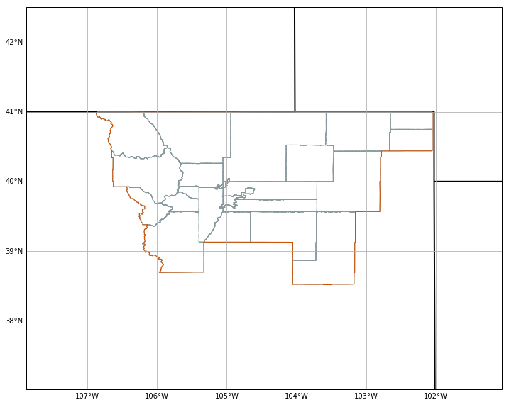
Using 25 county MultiPolygons

Create a merged CWA with cascaded_union

# Plot CWA envelope
for i, geom in enumerate(boundaries):
    gbounds = Polygon(geom)
    intersection = gbounds.intersection
    geoms = (intersection(geom)
         for geom in boundaries
         if gbounds.intersects(geom))
    shape_feature = ShapelyFeature(geoms,ccrs.PlateCarree(), 
                        facecolor='none', linestyle="-",linewidth=3.,edgecolor='#cc5000')
    ax.add_feature(shape_feature)

fig

WFO boundary spatial filter for interstates

Using the previously-defined envelope=merged_counties.buffer(2) in newDataRequest() to request geometries which fall inside the buffered boundary.

request = DataAccessLayer.newDataRequest('maps', envelope=envelope)
request.addIdentifier('table', 'mapdata.interstate')
request.addIdentifier('geomField', 'the_geom')
request.addIdentifier('locationField', 'hwy_type')
request.addIdentifier('hwy_type', 'I') # I (interstate), U (US highway), or S (state highway)
request.setParameters('name')
interstates = DataAccessLayer.getGeometryData(request, [])
print("Using " + str(len(interstates)) + " interstate MultiLineStrings")

# Plot interstates
for ob in interstates:
    shape_feature = ShapelyFeature(ob.getGeometry(),ccrs.PlateCarree(), 
                        facecolor='none', linestyle="-",edgecolor='orange')
    ax.add_feature(shape_feature)
fig

Using 223 interstate MultiLineStrings

Road type from select distinct(hwy_type) from mapdata.interstate;

    I - Interstates
    U - US Highways
    S - State Highways

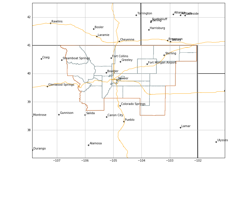
Nearby cities

Request the city table and filter by population and progressive disclosure level:

Warning: the prog_disc field is not entirely understood and values appear to change significantly depending on WFO site.

request = DataAccessLayer.newDataRequest('maps', envelope=envelope)
request.addIdentifier('table', 'mapdata.city')
request.addIdentifier('geomField', 'the_geom')
request.setParameters('name','population','prog_disc')
cities = DataAccessLayer.getGeometryData(request, [])
print("Found " + str(len(cities)) + " city Points")

Found 1201 city Points

citylist = []
cityname = []
# For BOU, progressive disclosure values above 50 and pop above 5000 looks good
for ob in cities:
    if ((ob.getNumber("prog_disc")>50) and int(ob.getString("population")) > 5000):
        citylist.append(ob.getGeometry())
        cityname.append(ob.getString("name"))
print("Using " + str(len(cityname)) + " city Points")

# Plot city markers
ax.scatter([point.x for point in citylist],
       [point.y for point in citylist],
       transform=ccrs.Geodetic(),marker="+",facecolor='black')
# Plot city names
for i, txt in enumerate(cityname):
    ax.annotate(txt, (citylist[i].x,citylist[i].y),
                xytext=(3,3), textcoords="offset points")

fig

Using 57 city Points

Lakes

request = DataAccessLayer.newDataRequest('maps', envelope=envelope)
request.addIdentifier('table', 'mapdata.lake')
request.addIdentifier('geomField', 'the_geom')
request.setParameters('name')

# Get lake geometries
response = DataAccessLayer.getGeometryData(request, [])
lakes = np.array([])
for ob in response:
    lakes = np.append(lakes,ob.getGeometry())
print("Using " + str(len(lakes)) + " lake MultiPolygons")

# Plot lakes
for i, geom in enumerate(lakes):
    cbounds = Polygon(geom)
    intersection = cbounds.intersection
    geoms = (intersection(geom)
         for geom in lakes
         if cbounds.intersects(geom))
    shape_feature = ShapelyFeature(geoms,ccrs.PlateCarree(), 
                        facecolor='blue', linestyle="-",edgecolor='#20B2AA')
    ax.add_feature(shape_feature)
fig

Using 208 lake MultiPolygons

Major Rivers

request = DataAccessLayer.newDataRequest('maps', envelope=envelope)
request.addIdentifier('table', 'mapdata.majorrivers')
request.addIdentifier('geomField', 'the_geom')
request.setParameters('pname')
rivers = DataAccessLayer.getGeometryData(request, [])
print("Using " + str(len(rivers)) + " river MultiLineStrings")

# Plot rivers
for ob in rivers:
    shape_feature = ShapelyFeature(ob.getGeometry(),ccrs.PlateCarree(), 
                        facecolor='none', linestyle=":",edgecolor='#20B2AA')
    ax.add_feature(shape_feature)
fig

Using 758 river MultiLineStrings

Topography

Spatial envelopes are required for topo requests, which can become slow to download and render for large (CONUS) maps.

import numpy.ma as ma
request = DataAccessLayer.newDataRequest()
request.setDatatype("topo")
request.addIdentifier("group", "/")
request.addIdentifier("dataset", "full")
request.setEnvelope(envelope)
gridData = DataAccessLayer.getGridData(request)
print(gridData)
print("Number of grid records: " + str(len(gridData)))
print("Sample grid data shape:\n" + str(gridData[0].getRawData().shape) + "\n")
print("Sample grid data:\n" + str(gridData[0].getRawData()) + "\n")

[<awips.dataaccess.PyGridData.PyGridData object at 0x1174adf50>]
Number of grid records: 1
Sample grid data shape:
(778, 1058)

Sample grid data:
[[ 1694.  1693.  1688. ...,   757.   761.   762.]
 [ 1701.  1701.  1701. ...,   758.   760.   762.]
 [ 1703.  1703.  1703. ...,   760.   761.   762.]
 ..., 
 [ 1767.  1741.  1706. ...,   769.   762.   768.]
 [ 1767.  1746.  1716. ...,   775.   765.   761.]
 [ 1781.  1753.  1730. ...,   766.   762.   759.]]

grid=gridData[0]
topo=ma.masked_invalid(grid.getRawData()) 
lons, lats = grid.getLatLonCoords()
print(topo.min())
print(topo.max())

# Plot topography
cs = ax.contourf(lons, lats, topo, 80, cmap=plt.get_cmap('terrain'),alpha=0.1)
cbar = fig.colorbar(cs, extend='both', shrink=0.5, orientation='horizontal')
cbar.set_label("topography height in meters")

fig

623.0
4328.0