8.3 KiB
8.3 KiB
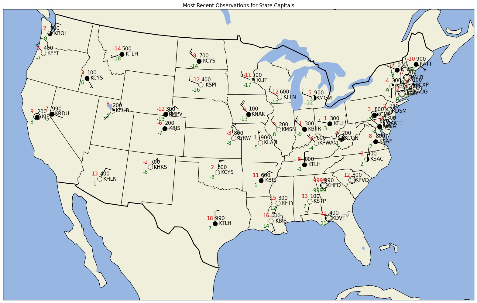
Based on the MetPy example "Station Plot with Layout"
import datetime
import pandas
import matplotlib.pyplot as plt
import numpy as np
import pprint
from awips.dataaccess import DataAccessLayer
from metpy.calc import get_wind_components
from metpy.cbook import get_test_data
from metpy.plots.wx_symbols import sky_cover, current_weather
from metpy.plots import StationPlot, StationPlotLayout, simple_layout
from metpy.units import units

def get_cloud_cover(code):
    if 'OVC' in code:
        return 1.0
    elif 'BKN' in code:
        return 6.0/8.0
    elif 'SCT' in code:
        return 4.0/8.0
    elif 'FEW' in code:
        return 2.0/8.0
    else:
        return 0

state_capital_wx_stations = {'Washington':'KOLM', 'Oregon':'KSLE', 'California':'KSAC',
                             'Nevada':'KCXP', 'Idaho':'KBOI', 'Montana':'KHLN',
                             'Utah':'KSLC', 'Arizona':'KDVT', 'New Mexico':'KSAF',
                             'Colorado':'KBKF', 'Wyoming':'KCYS', 'North Dakota':'KBIS',
                             'South Dakota':'KPIR', 'Nebraska':'KLNK', 'Kansas':'KTOP',
                             'Oklahoma':'KPWA', 'Texas':'KATT', 'Louisiana':'KBTR',
                             'Arkansas':'KLIT', 'Missouri':'KJEF', 'Iowa':'KDSM',
                             'Minnesota':'KSTP', 'Wisconsin':'KMSN', 'Illinois':'KSPI',
                             'Mississippi':'KHKS', 'Alabama':'KMGM', 'Nashville':'KBNA',
                             'Kentucky':'KFFT', 'Indiana':'KIND', 'Michigan':'KLAN',
                             'Ohio':'KCMH', 'Georgia':'KFTY', 'Florida':'KTLH',
                             'South Carolina':'KCUB', 'North Carolina':'KRDU',
                             'Virginia':'KRIC', 'West Virginia':'KCRW',
                             'Pennsylvania':'KCXY', 'New York':'KALB', 'Vermont':'KMPV',
                             'New Hampshire':'KCON', 'Maine':'KAUG', 'Massachusetts':'KBOS',
                             'Rhode Island':'KPVD', 'Connecticut':'KHFD', 'New Jersey':'KTTN',
                             'Delaware':'KDOV', 'Maryland':'KNAK'}
single_value_params = ["timeObs", "stationName", "longitude", "latitude",
                       "temperature", "dewpoint", "windDir",
                       "windSpeed", "seaLevelPress"]
multi_value_params = ["presWeather", "skyCover", "skyLayerBase"]
all_params = single_value_params + multi_value_params
obs_dict = dict({all_params: [] for all_params in all_params})
pres_weather = []
sky_cov = []
sky_layer_base = []
from dynamicserialize.dstypes.com.raytheon.uf.common.time import TimeRange
from datetime import datetime, timedelta
lastHourDateTime = datetime.utcnow() - timedelta(hours = 1)
start = lastHourDateTime.strftime('%Y-%m-%d %H')
beginRange = datetime.strptime( start + ":00:00", "%Y-%m-%d %H:%M:%S")
endRange = datetime.strptime( start + ":59:59", "%Y-%m-%d %H:%M:%S")
timerange = TimeRange(beginRange, endRange)
DataAccessLayer.changeEDEXHost("edex-cloud.unidata.ucar.edu")
request = DataAccessLayer.newDataRequest()
request.setDatatype("obs")
request.setParameters(*(all_params))
request.setLocationNames(*(state_capital_wx_stations.values()))
response = DataAccessLayer.getGeometryData(request,timerange)
for ob in response:
    avail_params = ob.getParameters()
    if "presWeather" in avail_params:
        pres_weather.append(ob.getString("presWeather"))
    elif "skyCover" in avail_params and "skyLayerBase" in avail_params:
        sky_cov.append(ob.getString("skyCover"))
        sky_layer_base.append(ob.getNumber("skyLayerBase"))
    else:
        for param in single_value_params:
            if param in avail_params:
                if param == 'timeObs':
                    obs_dict[param].append(datetime.fromtimestamp(ob.getNumber(param)/1000.0))
                else:
                    try:
                        obs_dict[param].append(ob.getNumber(param))
                    except TypeError:
                        obs_dict[param].append(ob.getString(param))
            else:
                obs_dict[param].append(None)

        obs_dict['presWeather'].append(pres_weather);
        obs_dict['skyCover'].append(sky_cov);
        obs_dict['skyLayerBase'].append(sky_layer_base);
        pres_weather = []
        sky_cov = []
        sky_layer_base = []
We can now use pandas to retrieve desired subsets of our observations.
In this case, return the most recent observation for each station.
df = pandas.DataFrame(data=obs_dict, columns=all_params)
#sort rows with the newest first
df = df.sort_values(by='timeObs', ascending=False)
#group rows by station
groups = df.groupby('stationName')
#create a new DataFrame for the most recent values
df_recent = pandas.DataFrame(columns=all_params)
#retrieve the first entry for each group, which will
#be the most recent observation
for rid, station in groups:
    row = station.head(1)
    df_recent = pandas.concat([df_recent, row])
Convert DataFrame to something metpy-readable by attaching units and calculating derived values
data = dict()
data['stid'] = np.array(df_recent["stationName"])
data['latitude']  = np.array(df_recent['latitude'])
data['longitude'] = np.array(df_recent['longitude'])
data['air_temperature'] = np.array(df_recent['temperature'], dtype=float)* units.degC
data['dew_point'] = np.array(df_recent['dewpoint'], dtype=float)* units.degC
data['slp'] = np.array(df_recent['seaLevelPress'])* units('mbar')
u, v = get_wind_components(np.array(df_recent['windSpeed']) * units('knots'),
                           np.array(df_recent['windDir']) * units.degree)
data['eastward_wind'], data['northward_wind'] = u, v
data['cloud_frac'] = [int(get_cloud_cover(x)*8) for x in df_recent['skyCover']]
%matplotlib inline
import cartopy.crs as ccrs
import cartopy.feature as feat
from matplotlib import rcParams
rcParams['savefig.dpi'] = 100
proj = ccrs.LambertConformal(central_longitude=-95, central_latitude=35,
                             standard_parallels=[35])
state_boundaries = feat.NaturalEarthFeature(category='cultural',
                                            name='admin_1_states_provinces_lines',
                                            scale='110m', facecolor='none')
# Create the figure
fig = plt.figure(figsize=(20, 15))
ax = fig.add_subplot(1, 1, 1, projection=proj)

# Add map elements
ax.add_feature(feat.LAND, zorder=-1)
ax.add_feature(feat.OCEAN, zorder=-1)
ax.add_feature(feat.LAKES, zorder=-1)
ax.coastlines(resolution='110m', zorder=2, color='black')
ax.add_feature(state_boundaries)
ax.add_feature(feat.BORDERS, linewidth='2', edgecolor='black')
ax.set_extent((-120, -70, 20, 50))

# Start the station plot by specifying the axes to draw on, as well as the
# lon/lat of the stations (with transform). We also set the fontsize to 12 pt.
stationplot = StationPlot(ax, data['longitude'], data['latitude'],
                          transform=ccrs.PlateCarree(), fontsize=12)

# The layout knows where everything should go, and things are standardized using
# the names of variables. So the layout pulls arrays out of `data` and plots them
# using `stationplot`.
simple_layout.plot(stationplot, data)

# Plot the temperature and dew point to the upper and lower left, respectively, of
# the center point. Each one uses a different color.
stationplot.plot_parameter('NW', np.array(data['air_temperature']), color='red')
stationplot.plot_parameter('SW', np.array(data['dew_point']), color='darkgreen')

# A more complex example uses a custom formatter to control how the sea-level pressure
# values are plotted. This uses the standard trailing 3-digits of the pressure value
# in tenths of millibars.
stationplot.plot_parameter('NE', np.array(data['slp']),
                           formatter=lambda v: format(10 * v, '.0f')[-3:])

# Plot the cloud cover symbols in the center location. This uses the codes made above and
# uses the `sky_cover` mapper to convert these values to font codes for the
# weather symbol font.
stationplot.plot_symbol('C', data['cloud_frac'], sky_cover)

# Also plot the actual text of the station id. Instead of cardinal directions,
# plot further out by specifying a location of 2 increments in x and 0 in y.
stationplot.plot_text((2, 0), np.array(obs_dict["stationName"]))

plt.title("Most Recent Observations for State Capitals")