Regional Surface Obs Plot
Notebook
This exercise creates a surface observsation station plot for the state
of Florida, using both METAR (datatype obs) and Synoptic (datatype
sfcobs). Because we are using the AWIPS Map Database for state and
county boundaries, there is no use of Cartopy cfeature in this
exercise.
from awips.dataaccess import DataAccessLayer
from dynamicserialize.dstypes.com.raytheon.uf.common.time import TimeRange
from datetime import datetime, timedelta
import numpy as np
import cartopy.crs as ccrs
from cartopy.mpl.gridliner import LONGITUDE_FORMATTER, LATITUDE_FORMATTER
from cartopy.feature import ShapelyFeature
from shapely.geometry import Polygon
import matplotlib.pyplot as plt
from metpy.units import units
from metpy.calc import wind_components
from metpy.plots import simple_layout, StationPlot, StationPlotLayout
import warnings
%matplotlib inline

def get_cloud_cover(code):
    if 'OVC' in code:
        return 1.0
    elif 'BKN' in code:
        return 6.0/8.0
    elif 'SCT' in code:
        return 4.0/8.0
    elif 'FEW' in code:
        return 2.0/8.0
    else:
        return 0
# EDEX request for a single state
edexServer = "edex-cloud.unidata.ucar.edu"
DataAccessLayer.changeEDEXHost(edexServer)
request = DataAccessLayer.newDataRequest('maps')
request.addIdentifier('table', 'mapdata.states')
request.addIdentifier('state', 'FL')
request.addIdentifier('geomField', 'the_geom')
request.setParameters('state','name','lat','lon')
response = DataAccessLayer.getGeometryData(request)
record = response[0]
print("Found " + str(len(response)) + " MultiPolygon")
state={}
state['name'] = record.getString('name')
state['state'] = record.getString('state')
state['lat'] = record.getNumber('lat')
state['lon'] = record.getNumber('lon')
#state['geom'] = record.getGeometry()
state['bounds'] = record.getGeometry().bounds
print(state['name'], state['state'], state['lat'], state['lon'], state['bounds'])
print()

# EDEX request for multiple states
request = DataAccessLayer.newDataRequest('maps')
request.addIdentifier('table', 'mapdata.states')
request.addIdentifier('geomField', 'the_geom')
request.addIdentifier('inLocation', 'true')
request.addIdentifier('locationField', 'state')
request.setParameters('state','name','lat','lon')
request.setLocationNames('FL','GA','MS','AL','SC','LA')
response = DataAccessLayer.getGeometryData(request)
print("Found " + str(len(response)) + " MultiPolygons")

# Append each geometry to a numpy array
states = np.array([])
for ob in response:
    print(ob.getString('name'), ob.getString('state'), ob.getNumber('lat'), ob.getNumber('lon'))
    states = np.append(states,ob.getGeometry())
Found 1 MultiPolygon
Florida FL 28.67402 -82.50934 (-87.63429260299995, 24.521051616000022, -80.03199876199994, 31.001012802000048)

Found 6 MultiPolygons
Florida FL 28.67402 -82.50934
Georgia GA 32.65155 -83.44848
Louisiana LA 31.0891 -92.02905
Alabama AL 32.79354 -86.82676
Mississippi MS 32.75201 -89.66553
South Carolina SC 33.93574 -80.89899
Now make sure we can plot the states with a lat/lon grid.
def make_map(bbox, proj=ccrs.PlateCarree()):
    fig, ax = plt.subplots(figsize=(16,12),subplot_kw=dict(projection=proj))
    ax.set_extent(bbox)
    gl = ax.gridlines(draw_labels=True, color='#e7e7e7')
    gl.top_labels = gl.right_labels = False
    gl.xformatter = LONGITUDE_FORMATTER
    gl.yformatter = LATITUDE_FORMATTER
    return fig, ax

# buffer our bounds by +/i degrees lat/lon
bounds = state['bounds']
bbox=[bounds[0]-3,bounds[2]+3,bounds[1]-1.5,bounds[3]+1.5]

fig, ax = make_map(bbox=bbox)
shape_feature = ShapelyFeature(states,ccrs.PlateCarree(),
                    facecolor='none', linestyle="-",edgecolor='#000000',linewidth=2)
ax.add_feature(shape_feature)
<cartopy.mpl.feature_artist.FeatureArtist at 0x11dcfedd8>

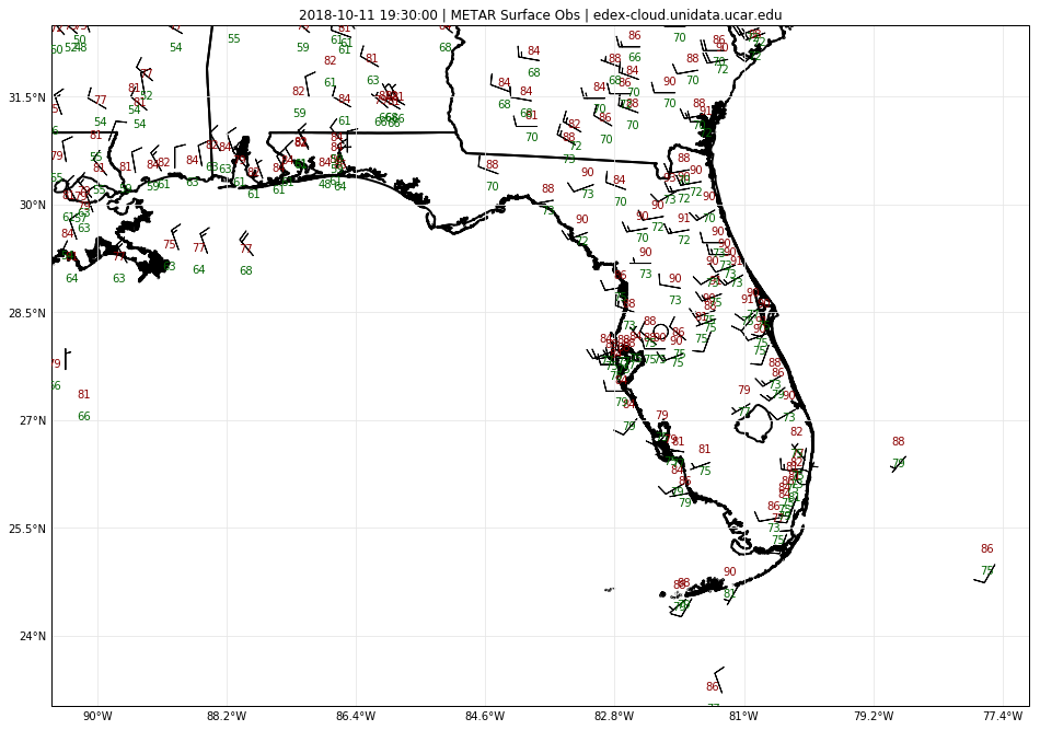
Plot METAR (obs)
Here we use a spatial envelope to limit the request to the boundary or our plot. Without such a filter you may be requesting many tens of thousands of records.
# Create envelope geometry
envelope = Polygon([(bbox[0],bbox[2]),(bbox[0],bbox[3]),
                    (bbox[1], bbox[3]),(bbox[1],bbox[2]),
                    (bbox[0],bbox[2])])

# New obs request
DataAccessLayer.changeEDEXHost(edexServer)
request = DataAccessLayer.newDataRequest("obs", envelope=envelope)
availableProducts = DataAccessLayer.getAvailableParameters(request)
single_value_params = ["timeObs", "stationName", "longitude", "latitude",
                       "temperature", "dewpoint", "windDir",
                       "windSpeed", "seaLevelPress"]
multi_value_params = ["presWeather", "skyCover", "skyLayerBase"]
params = single_value_params + multi_value_params
request.setParameters(*(params))

# Time range
lastHourDateTime = datetime.utcnow() - timedelta(minutes = 60)
start = lastHourDateTime.strftime('%Y-%m-%d %H:%M:%S')
end = datetime.utcnow().strftime('%Y-%m-%d %H:%M:%S')

beginRange = datetime.strptime( start , "%Y-%m-%d %H:%M:%S")
endRange = datetime.strptime( end , "%Y-%m-%d %H:%M:%S")
timerange = TimeRange(beginRange, endRange)
# Get response
response = DataAccessLayer.getGeometryData(request,timerange)
# function getMetarObs was added in python-awips 18.1.4
obs = DataAccessLayer.getMetarObs(response)
print("Found " + str(len(response)) + " records")
print("Using " + str(len(obs['temperature'])) + " temperature records")
Found 3468 records
Using 152 temperature records
Next grab the simple variables out of the data we have (attaching correct units), and put them into a dictionary that we will hand the plotting function later:
Get wind components from speed and direction
Convert cloud fraction values to integer codes [0 - 8]
Map METAR weather codes to WMO codes for weather symbols
data = dict()
data['stid'] = np.array(obs['stationName'])
data['latitude']  = np.array(obs['latitude'])
data['longitude'] = np.array(obs['longitude'])
tmp = np.array(obs['temperature'], dtype=float)
dpt = np.array(obs['dewpoint'], dtype=float)

# Suppress nan masking warnings
warnings.filterwarnings("ignore",category =RuntimeWarning)

tmp[tmp == -9999.0] = 'nan'
dpt[dpt == -9999.] = 'nan'
data['air_temperature'] = tmp * units.degC
data['dew_point_temperature'] = dpt * units.degC
data['air_pressure_at_sea_level'] = np.array(obs['seaLevelPress'])* units('mbar')
direction = np.array(obs['windDir'])
direction[direction == -9999.0] = 'nan'
u, v = wind_components(np.array(obs['windSpeed']) * units('knots'),
                           direction * units.degree)
data['eastward_wind'], data['northward_wind'] = u, v
data['cloud_coverage'] = [int(get_cloud_cover(x)*8) for x in obs['skyCover']]
data['present_weather'] = obs['presWeather']
proj = ccrs.LambertConformal(central_longitude=state['lon'], central_latitude=state['lat'],
                             standard_parallels=[35])
custom_layout = StationPlotLayout()
custom_layout.add_barb('eastward_wind', 'northward_wind', units='knots')
custom_layout.add_value('NW', 'air_temperature', fmt='.0f', units='degF', color='darkred')
custom_layout.add_value('SW', 'dew_point_temperature', fmt='.0f', units='degF', color='darkgreen')
custom_layout.add_value('E', 'precipitation', fmt='0.1f', units='inch', color='blue')
ax.set_title(str(response[-1].getDataTime()) + " | METAR Surface Obs | " + edexServer)
stationplot = StationPlot(ax, data['longitude'], data['latitude'], clip_on=True,
                          transform=ccrs.PlateCarree(), fontsize=10)
custom_layout.plot(stationplot, data)
fig
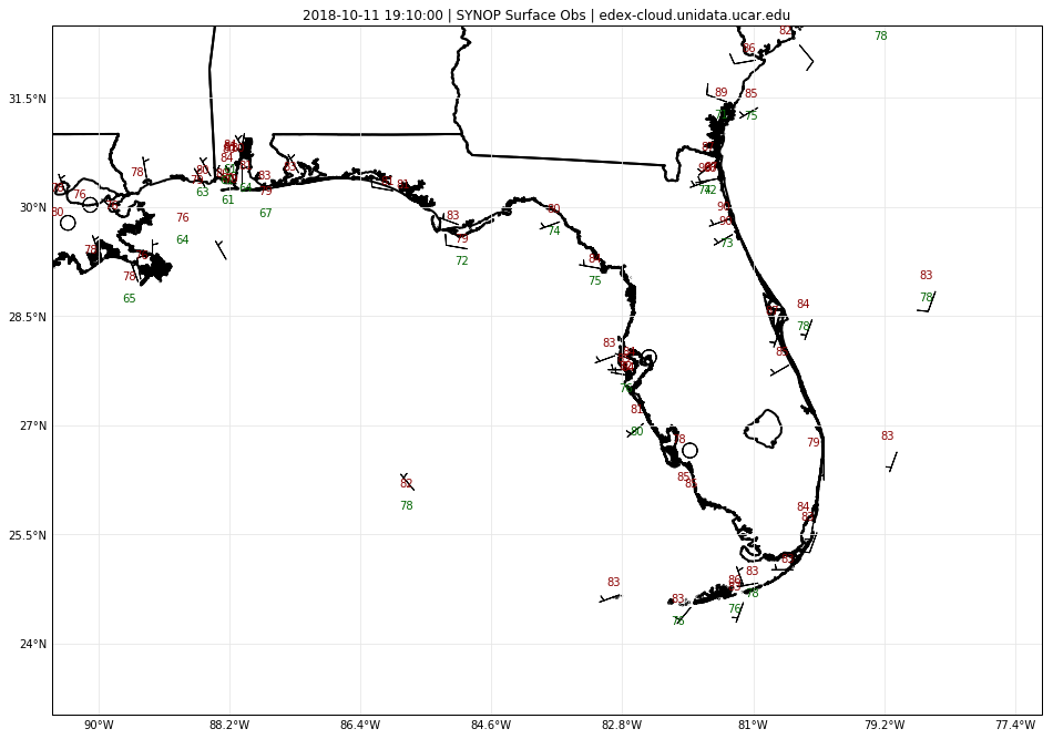
Plot Synoptic (sfcobs)
# New sfcobs/SYNOP request
DataAccessLayer.changeEDEXHost(edexServer)
request = DataAccessLayer.newDataRequest("sfcobs", envelope=envelope)
availableProducts = DataAccessLayer.getAvailableParameters(request)
# (sfcobs) uses stationId, while (obs) uses stationName,
# the rest of these parameters are the same.
single_value_params = ["timeObs", "stationId", "longitude", "latitude",
                       "temperature", "dewpoint", "windDir",
                       "windSpeed", "seaLevelPress"]
multi_value_params = ["presWeather", "skyCover", "skyLayerBase"]
pres_weather, sky_cov, sky_layer_base = [],[],[]
params = single_value_params + multi_value_params
request.setParameters(*(params))

# Time range
lastHourDateTime = datetime.utcnow() - timedelta(minutes = 60)
start = lastHourDateTime.strftime('%Y-%m-%d %H:%M:%S')
end = datetime.utcnow().strftime('%Y-%m-%d %H:%M:%S')

beginRange = datetime.strptime( start , "%Y-%m-%d %H:%M:%S")
endRange = datetime.strptime( end , "%Y-%m-%d %H:%M:%S")
timerange = TimeRange(beginRange, endRange)

# Get response
response = DataAccessLayer.getGeometryData(request,timerange)
# function getSynopticObs was added in python-awips 18.1.4
sfcobs = DataAccessLayer.getSynopticObs(response)
print("Found " + str(len(response)) + " records")
print("Using " + str(len(sfcobs['temperature'])) + " temperature records")
Found 260 records
Using 78 temperature records
data = dict()
data['stid'] = np.array(sfcobs['stationId'])
data['lat']  = np.array(sfcobs['latitude'])
data['lon'] = np.array(sfcobs['longitude'])

# Synop/sfcobs temps are stored in kelvin (degC for METAR/obs)
tmp = np.array(sfcobs['temperature'], dtype=float)
dpt = np.array(sfcobs['dewpoint'], dtype=float)
direction = np.array(sfcobs['windDir'])
# Account for missing values
tmp[tmp == -9999.0] = 'nan'
dpt[dpt == -9999.] = 'nan'
direction[direction == -9999.0] = 'nan'

data['air_temperature'] = tmp * units.kelvin
data['dew_point_temperature'] = dpt * units.kelvin
data['air_pressure_at_sea_level'] = np.array(sfcobs['seaLevelPress'])* units('mbar')
try:
    data['eastward_wind'], data['northward_wind'] = wind_components(
        np.array(sfcobs['windSpeed']) * units('knots'),direction * units.degree)
    data['present_weather'] = sfcobs['presWeather']
except ValueError:
    pass

fig_synop, ax_synop = make_map(bbox=bbox)
shape_feature = ShapelyFeature(states,ccrs.PlateCarree(),
                    facecolor='none', linestyle="-",edgecolor='#000000',linewidth=2)
ax_synop.add_feature(shape_feature)

custom_layout = StationPlotLayout()
custom_layout.add_barb('eastward_wind', 'northward_wind', units='knots')
custom_layout.add_value('NW', 'air_temperature', fmt='.0f', units='degF', color='darkred')
custom_layout.add_value('SW', 'dew_point_temperature', fmt='.0f', units='degF', color='darkgreen')
custom_layout.add_value('E', 'precipitation', fmt='0.1f', units='inch', color='blue')
ax_synop.set_title(str(response[-1].getDataTime()) + " | SYNOP Surface Obs | " + edexServer)
stationplot = StationPlot(ax_synop, data['lon'], data['lat'], clip_on=True,
                          transform=ccrs.PlateCarree(), fontsize=10)
custom_layout.plot(stationplot, data)
Plot both METAR and SYNOP
custom_layout = StationPlotLayout()
custom_layout.add_barb('eastward_wind', 'northward_wind', units='knots')
custom_layout.add_value('NW', 'air_temperature', fmt='.0f', units='degF', color='darkred')
custom_layout.add_value('SW', 'dew_point_temperature', fmt='.0f', units='degF', color='darkgreen')
custom_layout.add_value('E', 'precipitation', fmt='0.1f', units='inch', color='blue')
ax.set_title(str(response[-1].getDataTime()) + " | METAR/SYNOP Surface Obs | " + edexServer)
stationplot = StationPlot(ax, data['lon'], data['lat'], clip_on=True,
                          transform=ccrs.PlateCarree(), fontsize=10)
custom_layout.plot(stationplot, data)
fig
