METAR Station Plot with MetPy
Notebook This exercise creates a METAR plot for North America using AWIPS METAR observations (datatype obs) and MetPy.
from awips.dataaccess import DataAccessLayer
from dynamicserialize.dstypes.com.raytheon.uf.common.time import TimeRange
from datetime import datetime, timedelta
import numpy as np
import cartopy.crs as ccrs
import cartopy.feature as cfeature
import matplotlib.pyplot as plt
from metpy.calc import wind_components
from metpy.plots import StationPlot, StationPlotLayout
from metpy.units import units
import warnings
%matplotlib inline
warnings.filterwarnings("ignore",category =RuntimeWarning)

def get_cloud_cover(code):
    if 'OVC' in code:
        return 1.0
    elif 'BKN' in code:
        return 6.0/8.0
    elif 'SCT' in code:
        return 4.0/8.0
    elif 'FEW' in code:
        return 2.0/8.0
    else:
        return 0

# Pull out these specific stations (prepend K for AWIPS identifiers)
selected = ['PDX', 'OKC', 'ICT', 'GLD', 'MEM', 'BOS', 'MIA', 'MOB', 'ABQ', 'PHX', 'TTF',
            'ORD', 'BIL', 'BIS', 'CPR', 'LAX', 'ATL', 'MSP', 'SLC', 'DFW', 'NYC', 'PHL',
            'PIT', 'IND', 'OLY', 'SYR', 'LEX', 'CHS', 'TLH', 'HOU', 'GJT', 'LBB', 'LSV',
            'GRB', 'CLT', 'LNK', 'DSM', 'BOI', 'FSD', 'RAP', 'RIC', 'JAN', 'HSV', 'CRW',
            'SAT', 'BUY', '0CO', 'ZPC', 'VIH', 'BDG', 'MLF', 'ELY', 'WMC', 'OTH', 'CAR',
            'LMT', 'RDM', 'PDT', 'SEA', 'UIL', 'EPH', 'PUW', 'COE', 'MLP', 'PIH', 'IDA',
            'MSO', 'ACV', 'HLN', 'BIL', 'OLF', 'RUT', 'PSM', 'JAX', 'TPA', 'SHV', 'MSY',
            'ELP', 'RNO', 'FAT', 'SFO', 'NYL', 'BRO', 'MRF', 'DRT', 'FAR', 'BDE', 'DLH',
            'HOT', 'LBF', 'FLG', 'CLE', 'UNV']
selected = ['K{0}'.format(id) for id in selected]
data_arr = []
# EDEX Request
edexServer = "edex-cloud.unidata.ucar.edu"
DataAccessLayer.changeEDEXHost(edexServer)
request = DataAccessLayer.newDataRequest("obs")
availableProducts = DataAccessLayer.getAvailableParameters(request)

single_value_params = ["timeObs", "stationName", "longitude", "latitude",
                       "temperature", "dewpoint", "windDir",
                       "windSpeed", "seaLevelPress"]
multi_value_params = ["presWeather", "skyCover", "skyLayerBase"]
pres_weather, sky_cov, sky_layer_base = [],[],[]
params = single_value_params + multi_value_params
obs = dict({params: [] for params in params})

request.setParameters(*(params))
request.setLocationNames(*(selected))
Here we use the Python-AWIPS class TimeRange to prepare a beginning and end time span for requesting observations (the last hour):
# Time range
lastHourDateTime = datetime.utcnow() - timedelta(hours = 1)
start = lastHourDateTime.strftime('%Y-%m-%d %H')
beginRange = datetime.strptime( start + ":00:00", "%Y-%m-%d %H:%M:%S")
endRange = datetime.strptime( start + ":59:59", "%Y-%m-%d %H:%M:%S")
timerange = TimeRange(beginRange, endRange)

response = DataAccessLayer.getGeometryData(request,timerange)
station_names = []
for ob in response:
    avail_params = ob.getParameters()
    if "presWeather" in avail_params:
        pres_weather.append(ob.getString("presWeather"))
    elif "skyCover" in avail_params and "skyLayerBase" in avail_params:
        sky_cov.append(ob.getString("skyCover"))
        sky_layer_base.append(ob.getNumber("skyLayerBase"))
    else:
        # If we already have a record for this stationName, skip
        if ob.getString('stationName') not in station_names:
            station_names.append(ob.getString('stationName'))
            for param in single_value_params:
                if param in avail_params:
                    if param == 'timeObs':
                        obs[param].append(datetime.fromtimestamp(ob.getNumber(param)/1000.0))
                    else:
                        try:
                            obs[param].append(ob.getNumber(param))
                        except TypeError:
                            obs[param].append(ob.getString(param))
                else:
                    obs[param].append(None)

            obs['presWeather'].append(pres_weather);
            obs['skyCover'].append(sky_cov);
            obs['skyLayerBase'].append(sky_layer_base);
            pres_weather = []
            sky_cov = []
            sky_layer_base = []
Next grab the simple variables out of the data we have (attaching correct units), and put them into a dictionary that we will hand the plotting function later:
Get wind components from speed and direction
Convert cloud fraction values to integer codes [0 - 8]
Map METAR weather codes to WMO codes for weather symbols
data = dict()
data['stid'] = np.array(obs['stationName'])
data['latitude']  = np.array(obs['latitude'])
data['longitude'] = np.array(obs['longitude'])
data['air_temperature'] = np.array(obs['temperature'], dtype=float)* units.degC
data['dew_point_temperature'] = np.array(obs['dewpoint'], dtype=float)* units.degC
data['air_pressure_at_sea_level'] = np.array(obs['seaLevelPress'])* units('mbar')

direction = np.array(obs['windDir'])
direction[direction == -9999.0] = 'nan'

u, v = wind_components(np.array(obs['windSpeed']) * units('knots'),
                           direction * units.degree)
data['eastward_wind'], data['northward_wind'] = u, v
data['cloud_coverage'] = [int(get_cloud_cover(x)*8) for x in obs['skyCover']]
data['present_weather'] = obs['presWeather']
print(obs['stationName'])
['K0CO', 'KHOT', 'KSHV', 'KIND', 'KBDE', 'KPSM', 'KORD', 'KDFW', 'KPHL', 'KTTF', 'KBDG', 'KOLY', 'KNYC', 'KABQ', 'KLEX', 'KDRT', 'KELP', 'KRUT', 'KRIC', 'KPIT', 'KMSP', 'KHSV', 'KUNV', 'KSAT', 'KCLE', 'KPHX', 'KMIA', 'KBOI', 'KBRO', 'KLAX', 'KLBB', 'KMSO', 'KPDX', 'KTLH', 'KUIL', 'KTPA', 'KVIH', 'KBIL', 'KMLF', 'KCPR', 'KATL', 'KBIS', 'KCLT', 'KOKC', 'KRAP', 'KACV', 'KEPH', 'KELY', 'KFAR', 'KFAT', 'KMSY', 'KOLF', 'KPDT', 'KLMT', 'KHLN', 'KHOU', 'KICT', 'KIDA', 'KPIH', 'KPUW', 'KGJT', 'KGLD', 'KGRB', 'KLBF', 'KMLP', 'KBOS', 'KSYR', 'KDLH', 'KCOE', 'KOTH', 'KCRW', 'KSEA', 'KCAR', 'KDSM', 'KJAN', 'KSLC', 'KBUY', 'KLNK', 'KMEM', 'KNYL', 'KRDM', 'KCHS', 'KFSD', 'KJAX', 'KMOB', 'KRNO', 'KSFO', 'KWMC', 'KFLG', 'KLSV']
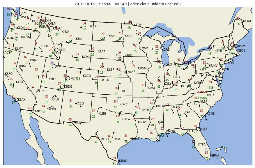
MetPy Surface Obs Plot
proj = ccrs.LambertConformal(central_longitude=-95, central_latitude=35,
                             standard_parallels=[35])

# Change the DPI of the figure
plt.rcParams['savefig.dpi'] = 255

# Winds, temps, dewpoint, station id
custom_layout = StationPlotLayout()
custom_layout.add_barb('eastward_wind', 'northward_wind', units='knots')
custom_layout.add_value('NW', 'air_temperature', fmt='.0f', units='degF', color='darkred')
custom_layout.add_value('SW', 'dew_point_temperature', fmt='.0f', units='degF', color='darkgreen')
custom_layout.add_value('E', 'precipitation', fmt='0.1f', units='inch', color='blue')

# Create the figure
fig = plt.figure(figsize=(20, 10))
ax = fig.add_subplot(1, 1, 1, projection=proj)

# Add various map elements
ax.add_feature(cfeature.LAND)
ax.add_feature(cfeature.OCEAN)
ax.add_feature(cfeature.LAKES)
ax.add_feature(cfeature.COASTLINE)
ax.add_feature(cfeature.STATES)
ax.add_feature(cfeature.BORDERS, linewidth=2)

# Set plot bounds
ax.set_extent((-118, -73, 23, 50))
ax.set_title(str(ob.getDataTime()) + " | METAR | " + edexServer)

stationplot = StationPlot(ax, data['longitude'], data['latitude'], clip_on=True,
                          transform=ccrs.PlateCarree(), fontsize=10)
stationplot.plot_text((2, 0), data['stid'])
custom_layout.plot(stationplot, data)
plt.show()